Phthalate Exposure in U.S. Women of Reproductive Age - an NHANES Review, Part II
Updated:
More fun with phthalates.
Motivation
In Part I of this post, we looked at what phthalates are, how humans interact with them, how much we have in our bodies, and how those levels have changed over time.
Here, we’ll attempt to answer Question 2:
- Are phthalate levels disproportionately distributed through the population? Namely, is there an association with phthalates and socioeconomic status?
For instance, do women with higher income have lower exposure to some/all phthalates. Or perhaps vice-versa? What about education? Why might this be the case? Well, it’s possible that phthalates like MEP are present predominantly in inexpensive consumer products, thereby increasing risk for women who purchase them. And because manufacturers are not required to disclose usage of phthalates (as discussed in our historical interlude above), it’s difficult to track them from the source. Understanding impacted groups gives us clues and insights into the mechanisms of action of these chemicals.
Analysis
We’ll be using the same datasets we used in Part I, and we’ll start here with the cleaned dataframe all_data_c (_c refers to creatinine-adjusted). Please refer back to Part I if something doesn’t make sense.
Libraries:
library(tidyverse)
library(stats)
library(viridis)
library(survey)
library(kableExtra)
library(gridExtra)
library(sjPlot)
Load in all_data_c:
all_data_c =
  readRDS("all_data_c.RDS")
Variables Used
SEQN: Unique NHANES identifierRIAGENDR: GenderRIDAGEYR: AgeRIDRETH1: EthnicityDMDEDUC2: EducationDMDMARTL: Marital StatusINDHHIN2: Annual household income (cycles 2007-2008, 2009-2010, 2011-2012, 2013-2014, 2015-2016)INDFMIN2: Annual family income (cycles 2007-2008, 2009-2010, 2011-2012, 2013-2014, 2015-2016)INDHHINC: Annual household income (cycles 2003-2004, 2005-2006)INDFMINC: Annual family income (cycles 2003-2004, 2005-2006)WTMEC2YR,SDMVPSU,SDMVSTRA: Survey weighting variables, addressed in Question 2 belowURXUCR: Urinary creatinineURXCNP: Mono(carboxyisononyl) phthalate (MCNP) (ng/mL)URXCOP: Mono(carboxyisoctyl) phthalate (MCOP) (ng/mL)URXMNP: Mono-isononyl phthalate (MiNP) (ng/mL)URXECP: Mono-2-ethyl-5-carboxypentyl phthalate (MECPP) (ng/mL)URXMHH: Mono-(2-ethyl-5-hydroxyhexyl) phthalate (MEHHP) (ng/mL)URXMHP: Mono-(2-ethyl)-hexyl phthalate (MEHP) (ng/mL)URXMOH: Mono-(2-ethyl-5-oxohexyl) phthalate (MEOHP) (ng/mL)URXMBP: Mono-n-butyl phthalate (MnBP) (ng/mL)URXMEP: Mono-ethyl phthalate (MEP) (ng/mL)URXMIB: Mono-isobutyl phthalate (MiBP) (ng/mL)URXMC1: Mono-(3-carboxypropyl) phthalate (MCPP) (ng/mL)URXMZP: Mono-benzyl phthalate (MBzP) (ng/mL)
Question 2: Are phthalate levels disproportionately distributed through the population? Namely, is there an association with phthalates and socioeconomic status?
Socioeconomic status is not a straightforward parameter to quantify. Often, it involves complex relationships between income, inherited wealth, education levels, race, and marital status. Because we are limited to the variables measured in NHANES, we will look at education as one proxy, and income as another.
To figure out the effects of these variables on phthalate levels, we will do two things. The first is an exploratory visualization (mostly because these are nice to look at), and the second is a more rigorous set of statistical regression models. But first, (of course) we have to do a bit more data manipulation.
Recode income and education variables
Income is measured in NHANES using two categorical variables, annual household income and annual family income. Both variables are coded using the same (somewhat non-intuitive) scale:
- 1: $0 - 4,999
- 2: $5,000 - 9,999
- 3: $10,000 - 14,999
- 4: $15,000 - 19,999
- 5: $20,000 - 24,999
- 6: $25,000 - 34,999
- 7: $35,000 - 44,999
- 8: $45,000 - 54,999
- 9: $55,000 - 64,999
- 10: $65,000 - 74,999
- 11: \(\ge\) $75,000 (2003-2004 and 2005-2006 cycles only)
- 12: \(\ge\) 20,000
- 13: < 20,000
- 14: $75,000 - 99,999 (2007-2008 cycles onward)
- 15: \(\ge\) $100,000
It’s not immediately clear which variable to use, but one would guess that they’re highly correlated. Indeed:
all_data_c %>%
  select(household_income, family_income) %>%
  cor(use = "complete.obs", method = "pearson")
##                  household_income family_income
## household_income        1.0000000     0.9095916
## family_income           0.9095916     1.0000000
Since the Pearson correlation coefficient is very high, we can choose either. I chose annual family income to account for younger women, or women that reside with family.
Next, I wanted to simplify analysis, make the levels more intuitive, and represent income levels in rough accordance with US class breakdown (poor, lower-middle class, middle and upper- middle class, and upper class). The income variable was collapsed into four annual income levels:
- level 1: < $20,000
- level 2: $20,000 - 45,000
- level 3: $45,000 - 100,000
- level 4: > $100,000
We will recode the education variable per the levels above, drop refused/don’t know/missing income observations, and ask R to interpret the variable type as categorical:
all_data_c =
  all_data_c %>%
  select(- household_income) %>%
  mutate(family_income =
           if_else(family_income %in% c(1:4, 13), 1,
                   if_else(family_income %in% c(5:7), 2,
                           if_else(family_income %in% c(8:11, 14), 3,
                                   if_else(family_income == 15, 4, 20)
                                   )
                           )
                   )
  ) %>%
  filter(!family_income %in% c(20, NA)) %>%
  mutate(family_income = as.factor(family_income))
Working with the education variable is a bit more straightforward. The NHANES categories for adults over 20 years of age are as follows:
- 1: < 9th grade
- 2: 9-11th grade
- 3: High school grad/GED
- 4: Some college/AA degree
- 5: College grad and above
Thus, all we need to do is drop the refuse/don’t know/missing education observations, fix the variable type to categorical, and we’re ready to roll.
all_data_c =
  all_data_c %>%
  drop_na(education) %>%
  filter(education %in% c(1:5)) %>%
  mutate(education = as.factor(education))
Visualization
Here we’ll look at some boxplots to eyeball trends. We won’t plot every phthalate because there’s a lot of them and the intent here is exploratory. Instead we’ll choose a handful of common ones, including those from both the low and high molecular weight categories.
# relabel education and income
box_plot_data =
all_data_c %>%
mutate(
education = recode(education, "1" = "< 9th grade", "2" = "< High school", "3" = "High school grad/GED", "4" = "Some college/AA degree", "5" = "College graduate and above", .default = NULL, .missing = NULL),
family_income = recode(family_income, "1" = "< $20,000", "2" = "$20,000 - 45,000", "3" = "$45,000 - 100,000 ", "4" = "> $100,000", .default = NULL, .missing = NULL)
)
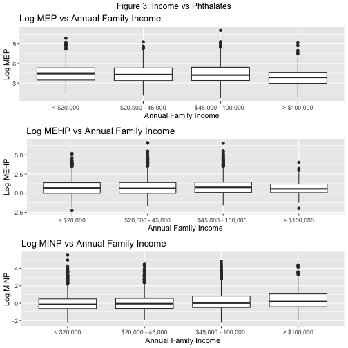
# income boxplots
mep_1 =
box_plot_data %>%
ggplot(aes(x = family_income, y = log(mep_c))) +
geom_boxplot() +
labs(
title = "Log MEP vs Annual Family Income",
x = "Annual Family Income",
y = "Log MEP"
)
mehp_1 =
box_plot_data %>%
ggplot(aes(x = family_income, y = log(mehp_c))) +
geom_boxplot() +
labs(
title = "Log MEHP vs Annual Family Income",
x = "Annual Family Income",
y = "Log MEHP"
)
minp_1 =
box_plot_data %>%
ggplot(aes(x = family_income, y = log(minp_c))) +
geom_boxplot() +
labs(
title = "Log MINP vs Annual Family Income",
x = "Annual Family Income",
y = "Log MINP"
)
grid.arrange(mep_1, mehp_1, minp_1, top = "Figure 3: Income vs Phthalates")
# education boxplots
mep_2 =
  box_plot_data %>%
    ggplot(aes(x = education, y = log(mep_c))) +
    geom_boxplot() +
    labs(
      title = "Log MEP vs Education",
      x = "Annual Family Income",
      y = "Log MEP"
    )

mehp_2 =
  box_plot_data %>%
    ggplot(aes(x = education, y = log(mehp_c))) +
    geom_boxplot() +
    labs(
      title = "Log MEHP vs Education",
      x = "Education",
      y = "Log MEHP"
    )

minp_2 =
  box_plot_data %>%
    ggplot(aes(x = family_income, y = log(minp_c))) +
    geom_boxplot() +
    labs(
      title = "Log MINP vs Education",
      x = "Education",
      y = "Log MINP"
    )

grid.arrange(mep_2, mehp_2, minp_2, top = "Figure 4: Education vs Phthalates")
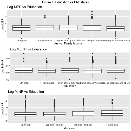
Admittedly, these boxplots are not as earth-shattering as I’d hoped. There’s definitely a lot of noise and not a definitive consistent pattern. But we can still glean some weak-ish trends. MEP biomarker levels show a slight decline with increasing income and education, MiNP shows the opposite trend, and MEHP fluctuates with both. We’ll need more rigorous analysis to pin-point relationships. Which means, it’s time to model.
Regression Models
The relationship between SES and phthalate levels is quantified below using multivariable linear regression models (a nice primer on regression modeling can be found here). Phthalates are modeled as outcome variables and are log-transformed to address the right-skew discussed above. Income and education are modeled as independent variables, and age is included as a covariate to adjust for potential confounding effects. Creatinine is added as a covariate to adjust for urine dilution.
This is where it gets a little tricky. NHANES uses a complex, stratified survey design (detailed here), along with over-sampling in accordance with the US census. Simply put, the ~10,000 individuals that participate in NHANES do not constitute a perfect random sample of the entire US population. Inevitably, some demographic groups will be over- or under-represented and some might not be represented at all. Therefore, each individual is assigned a sampling weight, which allows us to extrapolate results to the US population.
Because of this, it’s not enough to put the variables of interest into a model and hit play. Instead, we must utilize the survey package and the three survey variables, WTMEC2YR, SDMVPSU,SDMVSTRA that we’ve ignored up to now. The way these variables work is somewhat complicated and we won’t go into detail, but you can read all about it here. For our purposes, we need two steps: 1. create a survey design object using the survey variables and 2. carry out regression modeling using svyglm. This site provides a reference for both.
# adjust weighting variable for aggregation of 7 cycles
all_data_c$WTMEC14YR = all_data_c$WTMEC2YR/7

# create log variables
all_data_c =
  all_data_c %>%
  mutate(log_mecpp = log(mecpp),
         log_mnbp = log(mnbp),
         log_mcpp = log(mcpp),
         log_mep = log(mep),
         log_mehhp = log(mehhp),
         log_mehp = log(mehp),
         log_mibp = log(mibp),
         log_meohp = log(meohp),
         log_mbzp = log(mbzp),
         log_mcnp = log(mcnp),
         log_mcop = log(mcop),
         log_minp = log(minp)
         )

# selecting needed variables
all_data_m =
  all_data_c %>%
  filter(cycle %in% c("2003-2004","2005-2006","2007-2008","2009-2010","2011-2012", "2013-2014", "2015-2016")) %>%
  select(age, education, family_income, SDMVPSU, SDMVSTRA, WTMEC14YR, creatinine, log_mecpp, log_mnbp, log_mcpp, log_mep, log_mehhp, log_mehp, log_mibp, log_meohp, log_mbzp, log_mcnp, log_mcop, log_minp)

# create survey design variable
svy_design = svydesign(id = ~SDMVPSU, strata = ~SDMVSTRA, data = all_data_m, weights = ~WTMEC14YR, nest = TRUE)
Whew. Now we’re finally ready to model. Based on the variables we’re using, our theoretical model takes the following form. Note that because we have two multi-level categorical variables, we need to create n-1 “dummy” variables, n being the number of levels (more on dummy variables here).
\[ y_i = \beta_0 +\beta_1 * income_1 + \beta_2 * income_2 + \beta_3 * income_3 \] \[ + \beta_4 * education_1 + \beta_5 * education_2 + \beta_6 * education_3 \] \[ + \beta_7 * education_4 + \beta_8 * age + \beta_9 * creatinine + \epsilon_i \]
\(income_1 = {1\ for\ 20k-45k \ vs <20k, \ 0\ otherwise}\) \(income_2 = {1\ for\ 45k-100k \ vs <20k, \ 0\ otherwise}\) \(income_3 = {1\ for\ >100k\ vs <20k, \ 0\ otherwise}\) \(education_1 = {1\ for\ 9-11th\ grade \ vs <9th\ grade, \ 0\ otherwise}\) \(education_2 = {1\ for\ High\ school\ grad/GED \ vs <9th\ grade, \ 0\ otherwise}\) \(education_3 = {1\ for\ Some\ college/AA\ degree \ vs <9th\ grade, \ 0\ otherwise}\) \(education_4 = {1\ for\ College\ and\ above \ vs <9th\ grade, \ 0\ otherwise}\)
The fitted models are calculated below. It’ll be a lot of numbers but bear with me. We’ll get through it together.
mecpp_model = svyglm(log_mecpp ~ age + family_income + education + creatinine, design = svy_design, data = all_data_m)

mnbp_model = svyglm(log_mnbp ~ age + family_income + education + creatinine, design = svy_design, data = all_data_m)

mcpp_model = svyglm(log_mcpp ~ age + family_income + education + creatinine, design = svy_design, data = all_data_m)

mep_model = svyglm(log_mep ~ age + family_income + education + creatinine, design = svy_design, data = all_data_m)

mehhp_model = svyglm(log_mehhp ~ age + family_income + education + creatinine, design = svy_design, data = all_data_m)

mehp_model = svyglm(log_mehp ~ age + family_income + education + creatinine, design = svy_design, data = all_data_m)

mibp_model = svyglm(log_mibp ~ age + family_income + education + creatinine, design = svy_design, data = all_data_m)

meohp_model = svyglm(log_meohp ~ age + family_income + education + creatinine, design = svy_design, data = all_data_m)

mbzp_model = svyglm(log_mbzp ~ age + family_income + education + creatinine, design = svy_design, data = all_data_m)

mcnp_model = svyglm(log_mcnp ~ age + family_income + education + creatinine, design = svy_design, data = all_data_m)

mcop_model = svyglm(log_mcop ~ age + family_income + education + creatinine, design = svy_design, data = all_data_m)

minp_model = svyglm(log_minp ~ age + family_income + education + creatinine, design = svy_design, data = all_data_m)
# arranging models into tables
tab_model(mecpp_model, mnbp_model, mcpp_model, show.stat = TRUE, show.aic = FALSE, show.p = FALSE, title = "Table 2: Regression Results for MECPP, MnBP, and MCPP")
| log mecpp | log mnbp | log mcpp | |||||||
|---|---|---|---|---|---|---|---|---|---|
| Predictors | Estimates | CI | Statistic | Estimates | CI | Statistic | Estimates | CI | Statistic |
| (Intercept) | 2.24 | 1.89 – 2.58 | 12.67 | 1.28 | 0.92 – 1.63 | 7.08 | -0.37 | -0.74 – -0.00 | -1.97 |
| age | -0.00 | -0.01 – 0.00 | -0.79 | 0.01 | 0.00 – 0.02 | 2.45 | 0.00 | -0.01 – 0.01 | 0.25 |
| family_income [2] | -0.04 | -0.17 – 0.09 | -0.62 | -0.07 | -0.21 – 0.07 | -0.94 | -0.16 | -0.29 – -0.02 | -2.19 |
| family_income [3] | 0.17 | 0.03 – 0.32 | 2.31 | -0.11 | -0.27 – 0.04 | -1.42 | -0.13 | -0.26 – 0.01 | -1.78 |
| family_income [4] | -0.34 | -0.52 – -0.16 | -3.66 | -0.36 | -0.56 – -0.16 | -3.56 | -0.12 | -0.33 – 0.10 | -1.06 |
| education [2] | -0.19 | -0.44 – 0.06 | -1.51 | -0.02 | -0.25 – 0.21 | -0.17 | 0.10 | -0.14 – 0.34 | 0.84 |
| education [3] | -0.17 | -0.40 – 0.06 | -1.45 | -0.13 | -0.37 – 0.11 | -1.07 | 0.18 | -0.07 – 0.42 | 1.41 |
| education [4] | -0.22 | -0.44 – 0.01 | -1.89 | -0.15 | -0.39 – 0.09 | -1.23 | 0.21 | -0.03 – 0.46 | 1.68 |
| education [5] | -0.18 | -0.41 – 0.05 | -1.53 | -0.23 | -0.48 – 0.03 | -1.74 | 0.21 | -0.07 – 0.48 | 1.46 |
| creatinine | 0.01 | 0.01 – 0.01 | 20.68 | 0.01 | 0.01 – 0.01 | 29.62 | 0.01 | 0.01 – 0.01 | 24.35 |
| Observations | 2588 | 2588 | 2588 | ||||||
| R2 / R2 adjusted | 0.254 / -18.308 | 0.406 / -14.376 | 0.261 / -18.117 | ||||||
tab_model(mep_model, mehhp_model, mehp_model, show.stat = TRUE, show.aic = FALSE, show.p = FALSE, title = "Table 3: Regression Results for MEP, MEHHP, and MEHP")
| log mep | log mehhp | log mehp | |||||||
|---|---|---|---|---|---|---|---|---|---|
| Predictors | Estimates | CI | Statistic | Estimates | CI | Statistic | Estimates | CI | Statistic |
| (Intercept) | 2.47 | 1.99 – 2.95 | 10.12 | 1.51 | 1.15 – 1.88 | 8.14 | 0.27 | -0.06 – 0.59 | 1.60 |
| age | 0.02 | 0.01 – 0.03 | 4.11 | -0.00 | -0.01 – 0.01 | -0.12 | -0.01 | -0.01 – 0.00 | -1.40 |
| family_income [2] | -0.07 | -0.27 – 0.13 | -0.66 | -0.02 | -0.16 – 0.11 | -0.35 | 0.02 | -0.12 – 0.15 | 0.23 |
| family_income [3] | -0.05 | -0.28 – 0.18 | -0.41 | 0.17 | 0.02 – 0.33 | 2.21 | 0.13 | -0.01 – 0.26 | 1.87 |
| family_income [4] | -0.60 | -0.85 – -0.34 | -4.59 | -0.38 | -0.57 – -0.19 | -3.85 | -0.22 | -0.39 – -0.05 | -2.47 |
| education [2] | 0.11 | -0.18 – 0.41 | 0.74 | -0.11 | -0.36 – 0.14 | -0.85 | -0.17 | -0.40 – 0.06 | -1.47 |
| education [3] | 0.29 | -0.00 – 0.58 | 1.94 | -0.13 | -0.37 – 0.11 | -1.09 | -0.17 | -0.38 – 0.04 | -1.59 |
| education [4] | 0.15 | -0.16 – 0.47 | 0.94 | -0.11 | -0.34 – 0.12 | -0.94 | -0.19 | -0.38 – 0.00 | -1.92 |
| education [5] | -0.10 | -0.42 – 0.23 | -0.58 | -0.07 | -0.31 – 0.16 | -0.61 | -0.19 | -0.39 – 0.02 | -1.80 |
| creatinine | 0.01 | 0.01 – 0.01 | 19.20 | 0.01 | 0.01 – 0.01 | 22.05 | 0.01 | 0.01 – 0.01 | 19.73 |
| Observations | 2588 | 2588 | 2588 | ||||||
| R2 / R2 adjusted | 0.226 / -19.032 | 0.261 / -18.115 | 0.185 / -20.097 | ||||||
tab_model(mibp_model, meohp_model, mbzp_model, show.stat = TRUE, show.aic = FALSE, show.p = FALSE, title = "Table 4: Regression Results for MIBP, MEOHP, and MBZP")
| log mibp | log meohp | log mbzp | |||||||
|---|---|---|---|---|---|---|---|---|---|
| Predictors | Estimates | CI | Statistic | Estimates | CI | Statistic | Estimates | CI | Statistic |
| (Intercept) | 1.03 | 0.79 – 1.28 | 8.25 | 1.23 | 0.87 – 1.59 | 6.73 | 0.88 | 0.54 – 1.21 | 5.17 |
| age | -0.00 | -0.01 – 0.00 | -1.16 | -0.00 | -0.01 – 0.00 | -0.94 | -0.00 | -0.01 – 0.00 | -0.84 |
| family_income [2] | 0.06 | -0.05 – 0.17 | 1.13 | -0.02 | -0.15 – 0.12 | -0.23 | -0.07 | -0.19 – 0.06 | -1.05 |
| family_income [3] | -0.04 | -0.15 – 0.07 | -0.74 | 0.20 | 0.05 – 0.35 | 2.64 | -0.21 | -0.34 – -0.08 | -3.22 |
| family_income [4] | 0.04 | -0.12 – 0.19 | 0.44 | -0.39 | -0.57 – -0.20 | -4.05 | -0.59 | -0.76 – -0.42 | -6.90 |
| education [2] | -0.13 | -0.33 – 0.06 | -1.32 | -0.17 | -0.42 – 0.08 | -1.36 | 0.26 | 0.03 – 0.50 | 2.19 |
| education [3] | -0.36 | -0.56 – -0.17 | -3.68 | -0.17 | -0.41 – 0.07 | -1.40 | 0.04 | -0.19 – 0.27 | 0.34 |
| education [4] | -0.29 | -0.46 – -0.12 | -3.28 | -0.17 | -0.40 – 0.05 | -1.49 | 0.07 | -0.15 – 0.28 | 0.61 |
| education [5] | -0.28 | -0.47 – -0.10 | -2.96 | -0.10 | -0.34 – 0.14 | -0.85 | -0.14 | -0.37 – 0.10 | -1.16 |
| creatinine | 0.01 | 0.01 – 0.01 | 34.30 | 0.01 | 0.01 – 0.01 | 22.93 | 0.01 | 0.01 – 0.01 | 31.87 |
| Observations | 2588 | 2588 | 2588 | ||||||
| R2 / R2 adjusted | 0.430 / -13.757 | 0.282 / -17.585 | 0.414 / -14.169 | ||||||
tab_model(mcnp_model, mcop_model, minp_model, show.stat = TRUE, show.aic = FALSE, show.p = FALSE, title = "Table 5: Regression Results for MCNP, MCOP, and MINP")
| log mcnp | log mcop | log minp | |||||||
|---|---|---|---|---|---|---|---|---|---|
| Predictors | Estimates | CI | Statistic | Estimates | CI | Statistic | Estimates | CI | Statistic |
| (Intercept) | 0.03 | -0.32 – 0.37 | 0.16 | 1.75 | 1.33 – 2.16 | 8.28 | -0.10 | -0.38 – 0.18 | -0.69 |
| age | -0.01 | -0.01 – 0.00 | -1.70 | -0.01 | -0.02 – -0.00 | -2.52 | -0.01 | -0.01 – 0.00 | -1.54 |
| family_income [2] | -0.09 | -0.21 – 0.03 | -1.46 | -0.06 | -0.28 – 0.16 | -0.51 | -0.03 | -0.14 – 0.09 | -0.47 |
| family_income [3] | -0.00 | -0.13 – 0.12 | -0.08 | -0.07 | -0.27 – 0.13 | -0.70 | -0.01 | -0.14 – 0.11 | -0.18 |
| family_income [4] | -0.05 | -0.23 – 0.14 | -0.50 | 0.15 | -0.12 – 0.42 | 1.10 | 0.02 | -0.16 – 0.21 | 0.24 |
| education [2] | 0.04 | -0.20 – 0.27 | 0.33 | -0.09 | -0.38 – 0.20 | -0.59 | -0.05 | -0.22 – 0.13 | -0.52 |
| education [3] | 0.11 | -0.09 – 0.32 | 1.07 | 0.01 | -0.30 – 0.32 | 0.07 | 0.07 | -0.10 – 0.23 | 0.83 |
| education [4] | 0.17 | -0.04 – 0.37 | 1.62 | 0.09 | -0.20 – 0.37 | 0.61 | 0.09 | -0.08 – 0.26 | 0.99 |
| education [5] | 0.26 | 0.02 – 0.51 | 2.10 | 0.15 | -0.16 – 0.47 | 0.95 | 0.10 | -0.08 – 0.29 | 1.11 |
| creatinine | 0.01 | 0.01 – 0.01 | 19.74 | 0.01 | 0.01 – 0.01 | 16.41 | 0.00 | 0.00 – 0.00 | 9.03 |
| Observations | 2225 | 2225 | 2588 | ||||||
| R2 / R2 adjusted | 0.260 / -18.368 | 0.171 / -20.687 | 0.051 / -23.553 | ||||||
Let’s dissect the results. If we look at income first, we see generally negative values for the parameter estimates. This signals that higher income generally corresponds with lower urinary phthalate concentration. The parameters are pretty small and most are not statistically significant at an alpha level of 0.05. Notably, at the highest family income category, family_income_4 (meaning the highest earners vs the lowest earners), the estimates tend to be higher and most of them are statistically significant. This means that, in general, there is only an association between annual family income and phthalate exposure at the extremes of income.
Looking at education, we also see very small estimates for the beta parameters and almost all of them are not statistically significant.
So is there an association between socioeconomic status and phthalate exposure? Eh… not really. (I know, that’s a very scientific answer.) There are some weak relationships but based on data gathered from 13 years of observation, phthalates seem to be everywhere and permeate all levels of society. But hey, at least we know they’ve decreased from the early 2000s.
Conlusions
Wasn’t that fun?? I had fun. In addition to our conclusions from Part I, we learned that:
- Multivariable regression modeling did not establish strong associations between phthalate exposure and measures of socioeconomic status.
I hope you agree that we’ve learned a lot of good stuff. It’s clear to me that we don’t really understand the full story. Research on phthalates didn’t start until the early 2000s and plastics themselves are a relatively young addition to the human toolkit. So there’s no question that further work needs to be done. Until then, I feel a little less anxious about phthalates.
Still, I will definitely not be sticking plastic in the microwave and if you’re pregnant, you probably shouldn’t either.
Thank you for reading. Comments and questions are always welcome.
Further Reading
For more than you ever wanted to know about phthalates, check out this publicly available report published by the National Academies and this document published by the EPA. For something a bit more entertaining, The Guardian published this pretty comprehensive article in 2015.
References
- Zota, Ami R., et al. “Temporal Trends in Phthalate Exposures: Findings from the National Health and Nutrition Examination Survey, 2001–2010.” Environmental Health Perspectives, vol. 122, no. 3, 2014, pp. 235–241., doi:10.1289/ehp.1306681.
- Polańska, Kinga, et al. “Effect of Environmental Phthalate Exposure on Pregnancy Duration and Birth Outcomes.” International Journal of Occupational Medicine and Environmental Health, vol. 29, no. 4, 2016, pp. 683–697., doi:10.13075/ijomeh.1896.00691.
- Swan, Shanna H. “Environmental Phthalate Exposure in Relation to Reproductive Outcomes and Other Health Endpoints in Humans.” Environmental Research, vol. 108, no. 2, 2008, pp. 177–184., doi:10.1016/j.envres.2008.08.007.
- Duty, Susan M, et al. “The Relationship between Environmental Exposures to Phthalates and DNA Damage in Human Sperm Using the Neutral Comet Assay.” Environmental Health Perspectives, vol. 111, no. 9, 2003, pp. 1164–1169., doi:10.1289/ehp.5756.
- Sciences, Roundtable on Environmental Health, et al. “The Challenge: Chemicals in Today’s Society.” Identifying and Reducing Environmental Health Risks of Chemicals in Our Society: Workshop Summary., U.S. National Library of Medicine, 2 Oct. 2014, www.ncbi.nlm.nih.gov/books/NBK268889/.
- Lyche, Jan L., et al. “Reproductive and Developmental Toxicity of Phthalates.” Journal of Toxicology and Environmental Health, Part B, vol. 12, no. 4, 2009, pp. 225–249., doi:10.1080/10937400903094091.
- NTP-CERHR Expert Panel Update on the Reproductive and Developmental Toxicity of Di(2-Ethylhexyl) Phthalate.” Reproductive Toxicology, vol. 22, no. 3, 2006, pp. 291–399., doi:10.1016/j.reprotox.2006.04.007.
- Grande, Simone Wichert, et al. “A Dose-Response Study Following In Utero and Lactational Exposure to Di(2-Ethylhexyl)Phthalate: Effects on Female Rat Reproductive Development.” Toxicological Sciences, vol. 91, no. 1, 2006, pp. 247–254., doi:10.1093/toxsci/kfj128.